physicskit

Package
Quality
Documentation
Code style
Downloads
Community

Watch the laws of physics play out. physicskit is a Python toolkit for learning and teaching computational physics, spanning the field end to end: the quantum mechanics of a single hydrogen atom, the numerical relativity of colliding black holes, turbulent fluid instabilities, topological insulators, magnetically confined plasmas, and chaotic quantum billiards. Every simulation keeps its full trajectory, every domain ships plotting and animation helpers, and each domain's docs walk through the field's breakthroughs in historical order, each one linked to runnable code that reproduces it.

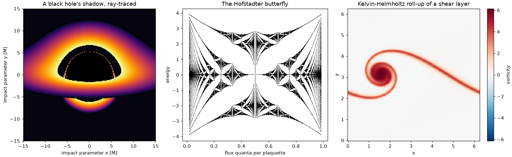
• For students: send a wave packet through a double slit, watch edge states cross a topological band gap, trace light around a black hole, all in a few lines each.
• For instructors: 14 domains, one consistent API, and over 300 gallery examples, each downloadable as a Python script or Jupyter notebook, ready to hand out as course material.
• Built on numpy/scipy: library routines under the hood, numba-compiled inner loops where the physics is time-stepped, and algorithms hand-rolled only where the steps themselves are what you're learning (see Design).

physicskit is part of a family of packages -- physicskit, mathematicskit and chemistrykit -- that share the same architecture, API conventions, and history-driven documentation. For tight-binding models beyond physicskit.condensed -- arbitrary finite lattices, ribbons and defects, non-Hermitian bands, Landauer transport, and the kernel polynomial method for very large samples -- see the dedicated package tbkit.

Install

pip install physicskit

Then import physicskit as pk. Runtime dependencies are numpy, scipy, matplotlib, numba (which compiles the shared integrators and the time-stepping loops of chaos, classical, fluids, plasma, relativity, and statphys), plotly, sympy, and tqdm. The interactive 3D viewer in physicskit.chaos.visualizers.viewer3d additionally needs pip install pyvista.

For development: pip install -e ".[dev]" (see CONTRIBUTING.md).

Quick start

import numpy as np
import matplotlib.pyplot as plt
import physicskit as pk

# The Haldane model's two bands carry Chern numbers +1 and -1...
H = lambda k1, k2: pk.condensed.haldane_model(k1, k2, phi=np.pi / 2)
print(pk.condensed.compute_chern_number(H, grid_size=30))  # [1, -1]

# ...so a finite ribbon has chiral edge states crossing the bulk gap
bulk = pk.condensed.haldane_lattice_hamiltonian(t2=0.2, phi=np.pi / 2)
ribbon = pk.condensed.build_ribbon(bulk, open_direction=1, n_cells=20)
k = np.linspace(0, 2 * np.pi, 200)
plt.plot(k, [np.linalg.eigvalsh(ribbon([kk])) for kk in k], color="C0", lw=0.8)

Every subpackage below links to its worked examples, or browse the docs at https://cpoli.github.io/physicskit/.

Subpackages

Domain subpackages, each with runnable examples linked below:

• physicskit.astro -- stellar structure (Lane-Emden polytropes, Tolman-Oppenheimer-Volkoff, the Chandrasekhar limit), N-body dynamics with symplectic integrators (including the figure-eight choreography), Keplerian orbital mechanics and Hohmann transfers, galactic rotation curves and NFW dark-matter halos, Zel'dovich cosmic-web formation (numpy.fft), and stellar convection with an alpha-omega magnetic dynamo.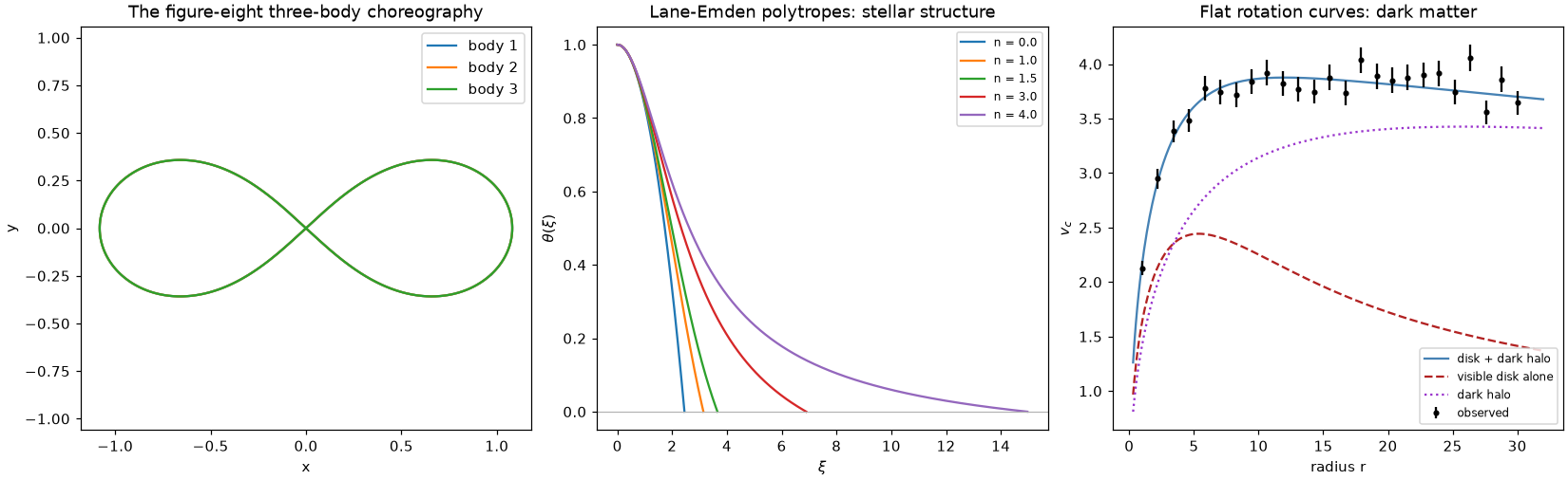

  

• physicskit.chaos -- chaotic dynamical systems: continuous flows (Lorenz, Rössler, Duffing, Chua, double and magnetic pendulums), discrete maps (logistic, Hénon, standard, baker's, Smale horseshoe), classical billiards (circle, ellipse, stadium, Sinai), Lyapunov spectra by Benettin's QR method, fractal dimensions and recurrence analysis, and 2D quantum billiards and kicked rotors (numba-compiled flows and maps; quantum billiard eigenstates via scipy.sparse.linalg.eigsh).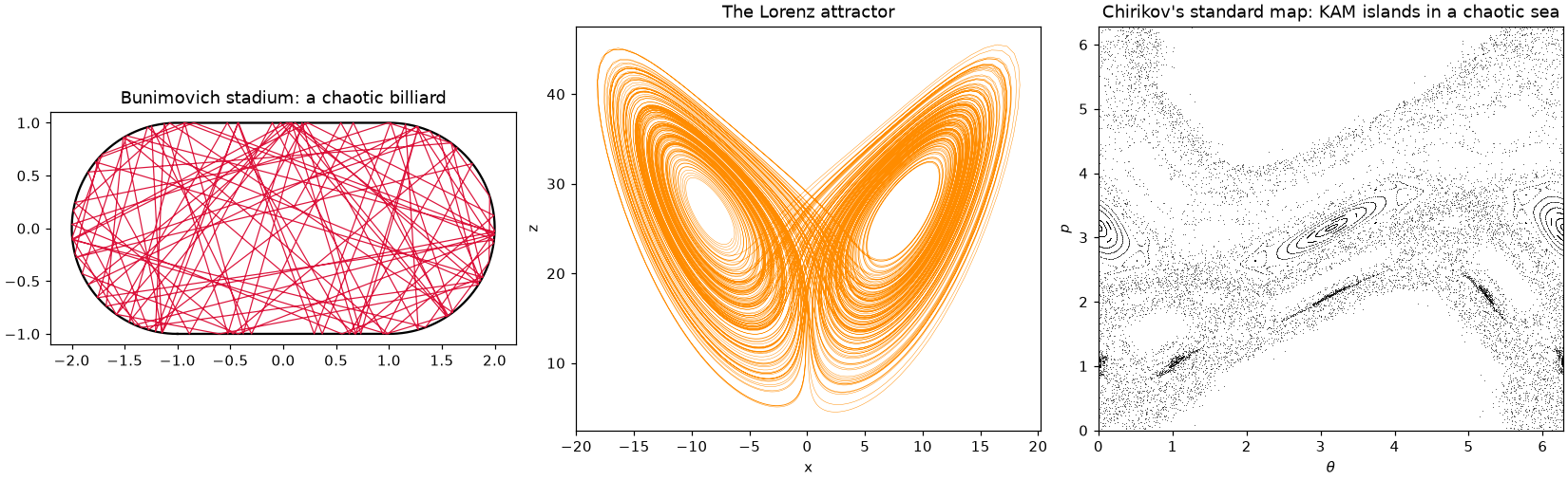

  

• physicskit.classical -- classical mechanics: Newtonian, Lagrangian (with a symbolic equations-of-motion engine), Hamiltonian, lattice, and rigid-body dynamics -- the FPUT recurrence, Hénon-Heiles and KAM tori, the double and elastic pendulums, the Foucault pendulum, and the Dzhanibekov effect, Euler's disk, and the rattleback (numba-compiled symplectic and implicit-midpoint integrators).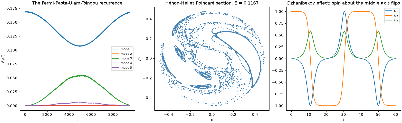

  

• physicskit.condensed -- tight-binding models (Bloch bands, Slater-Koster, Peierls substitution and the Hofstadter butterfly), topological band theory (Chern numbers, Zak phase, Z2 invariants, the tenfold way, SSH/Haldane/Kane-Mele/Kitaev/Weyl edge and surface states), Anderson localization, Landau levels and the quantum Hall effects, correlated electrons (BCS, Hubbard, Ginzburg-Landau), exact diagonalization of quantum spin chains (Bethe ansatz, transverse-field Ising, entanglement scaling), phonons and the Debye heat capacity, and Drude/Boltzmann transport (diagonalization via numpy.linalg.eigh).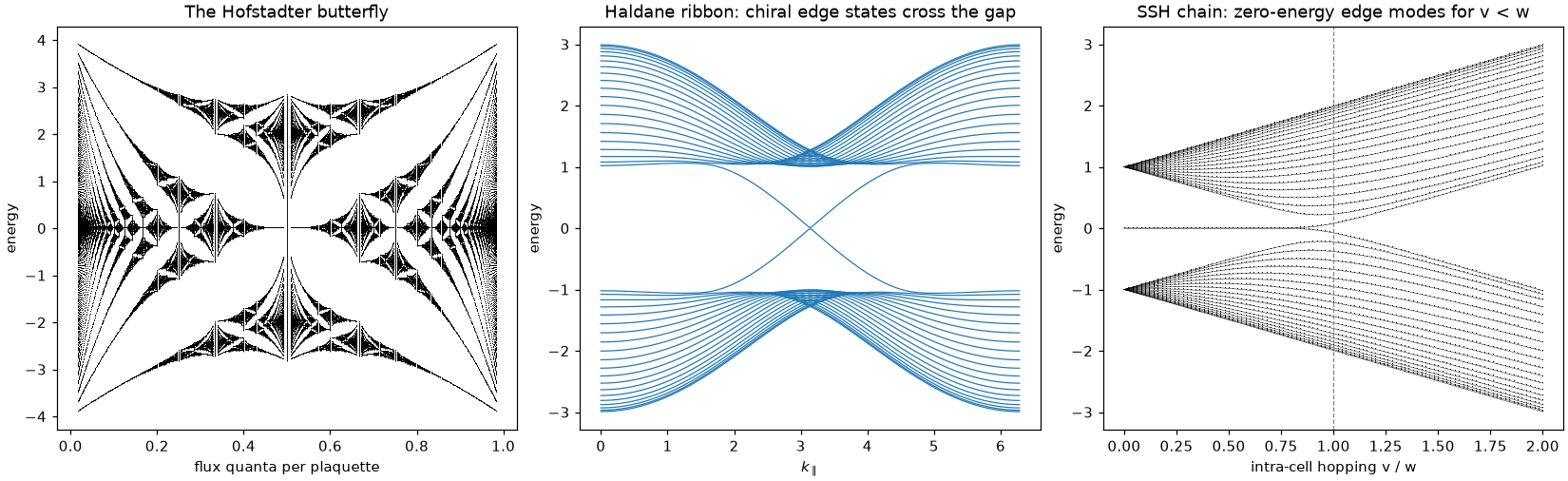

  

• physicskit.fields -- electrostatics (Poisson solvers, the method of images, multipole expansions) and Biot-Savart magnetostatics, FDTD electrodynamics on the Yee grid with perfectly matched layers, KdV/NLS/Sine-Gordon solitons (split-step spectral methods via numpy.fft), and Gross-Pitaevskii Bose-Einstein condensates with quantized vortices and vortex lattices.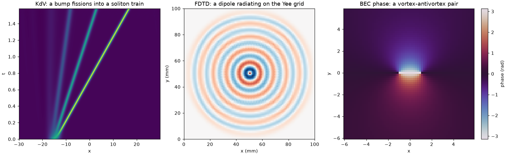

  

• physicskit.fluids -- potential flow (sources, doublets, Kutta-Joukowski lift), viscous exact solutions (Couette, Poiseuille, Blasius, Stokes drag), point-vortex dynamics and the von Kármán street, Kelvin-Helmholtz and Rayleigh-Taylor instabilities, compressible shocks (the Sod shock tube), the 2D incompressible Navier-Stokes solver underlying them (pseudo-spectral via numpy.fft, numba-compiled vortex kernels), linear continuum mechanics (heat equation, acoustics, 2D elasticity), and a D2Q9 lattice Boltzmann solver.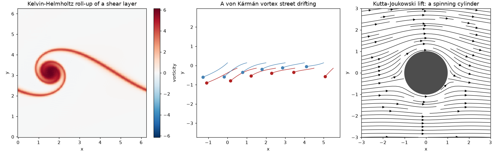

  

• physicskit.optics -- ray optics and ABCD matrices, Fresnel/Fraunhofer wave optics (numpy.fft), Gaussian and Laguerre-Gauss beams (scipy.special), and quantum optics (coherent and squeezed states, photon statistics, the Jaynes-Cummings model, Wigner functions), and lasers (rate equations and Maxwell-Bloch dynamics).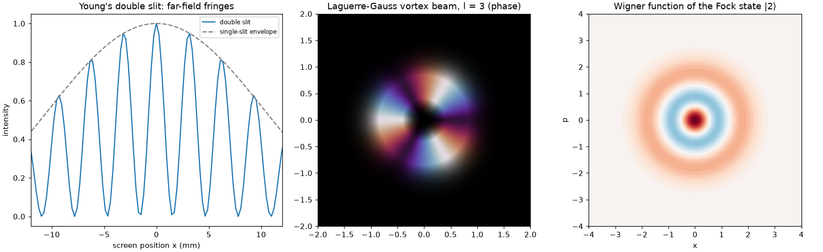

  

• physicskit.particle -- relativistic kinematics (four-vectors, boosts, Mandelstam variables), particle decays and scattering, detector signatures and resonance searches (from the J/psi to the Higgs), weak interactions and neutrino oscillations, radioactive decay chains, nuclear physics (Rutherford scattering, the semi-empirical mass formula, fission), and U(1) lattice gauge theory with Wilson loops.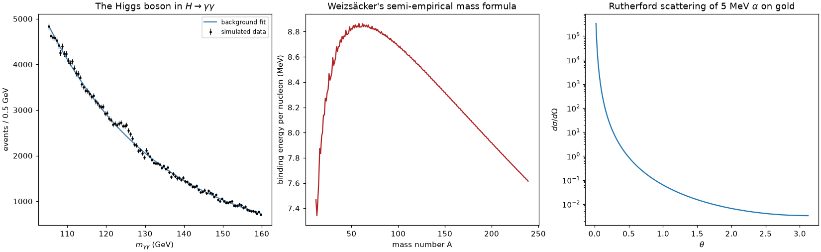

  

• physicskit.plasma -- Boris-pusher single-particle motion, guiding-center drifts and magnetic mirrors, Grad-Shafranov MHD equilibrium, magnetic reconnection, cold-plasma wave dispersion and the CMA diagram, particle-in-cell Vlasov-Poisson kinetics (Landau damping, two-stream and Weibel instabilities), and Hasegawa-Mima drift-wave turbulence (numba-compiled particle pushers, spectral field solves via numpy.fft).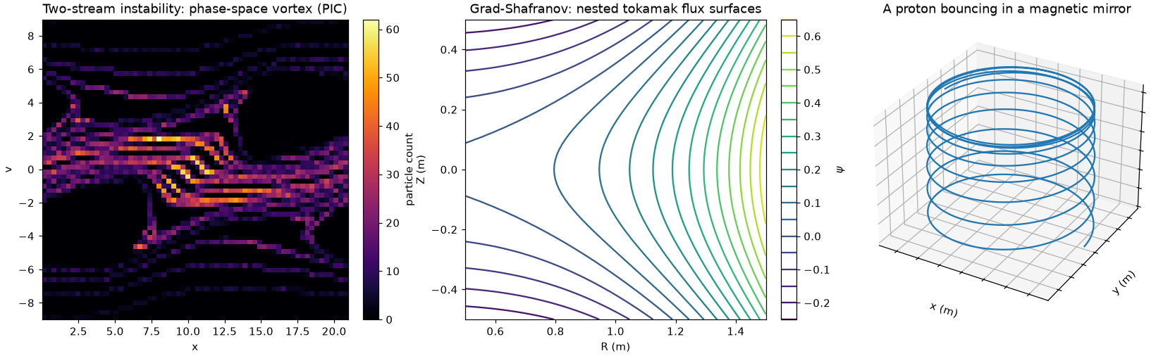

  

• physicskit.quantum -- quantum mechanics: wave packets (split-operator propagation via numpy.fft), potentials and tunneling (matrix Numerov and sparse eigensolvers via scipy.sparse.linalg.eigsh), hydrogen and angular momentum, entanglement and Bell inequalities, measurement (Born rule, Stern-Gerlach, the double slit), perturbation and Floquet theory, open systems (Lindblad, quantum trajectories), the Dirac and Klein-Gordon equations, Born and partial-wave scattering, and Hartree-Fock.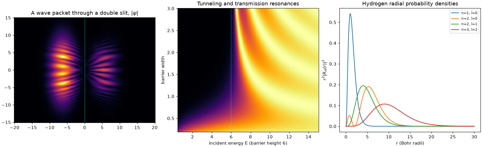

  

• physicskit.relativity -- numerical general relativity: Schwarzschild and Kerr geodesics (numba-compiled), ray-traced black hole shadows, gravitational lensing, gravitational waves from binary inspiral to merger and ringdown, neutron stars (TOV), FLRW cosmology, and a numerical curvature engine validated against Einstein's vacuum field equations, with ADM initial data.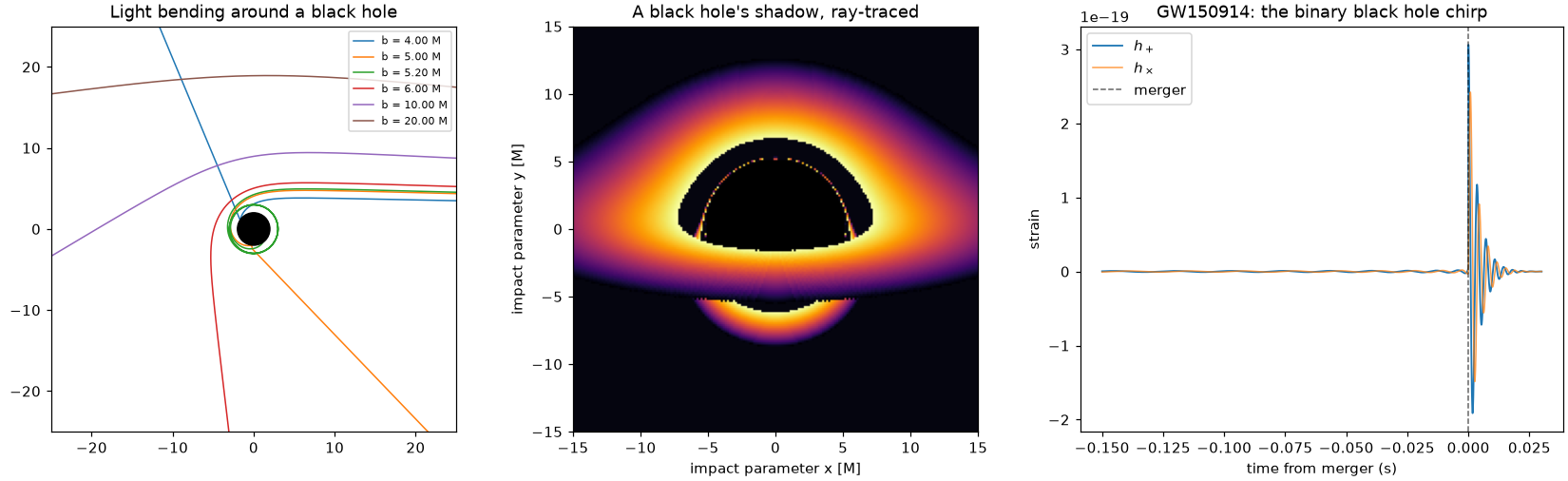

  

• physicskit.rmt -- random matrix theory, organized around Dyson's threefold way: Gaussian, circular, Ginibre, Wishart, and Bogoliubov-de Gennes ensembles, with each classic law (semicircle, Wigner surmise, Tracy-Widom, Marchenko-Pastur, circular law, ...) validated against its closed form (numpy.linalg eigensolvers, scipy.stats Kolmogorov-Smirnov tests).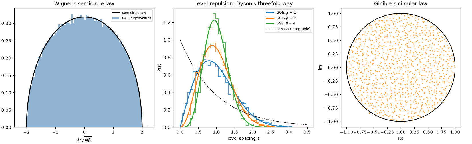

  

• physicskit.semiclassical -- WKB/EBK quantization and Maslov indices, Van Vleck/Herman-Kluk semiclassical propagators, Feynman's path integral and its classical limit, the Gutzwiller and Berry-Tabor trace formulas, and quantum scarring.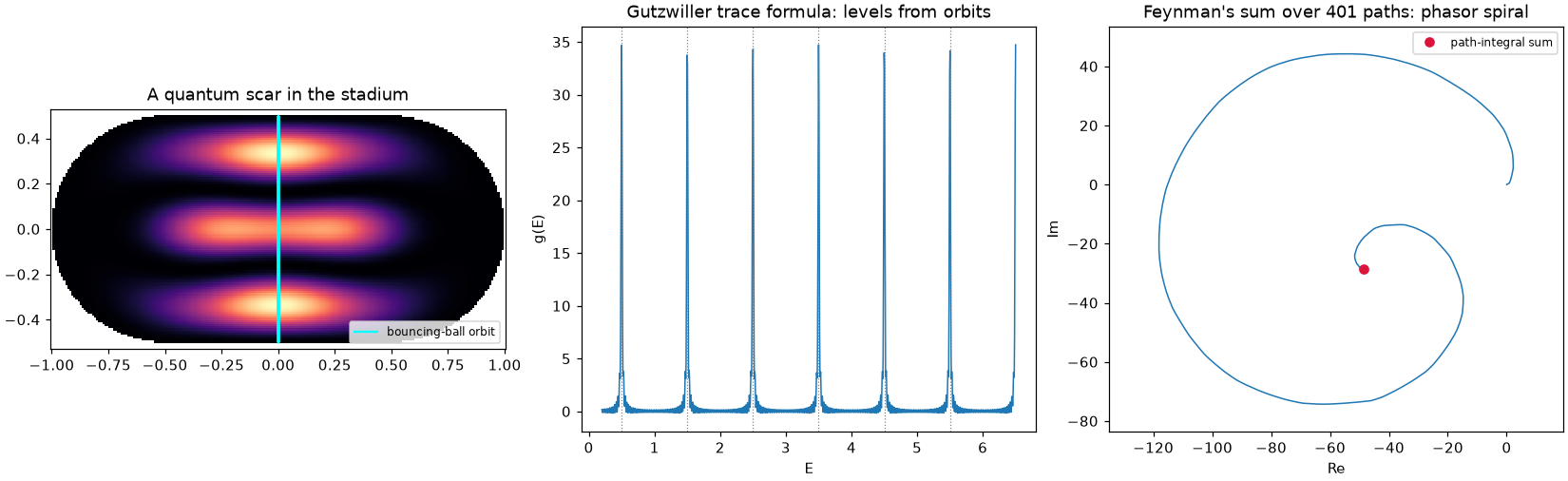

  

• physicskit.statphys -- statistical mechanics: Ising, Potts, and XY lattice models (numba-compiled Metropolis and Wolff cluster updates), molecular dynamics, criticality and the renormalization group, percolation, self-organized criticality, KPZ growth, spin glasses, Lee-Yang zeros, nonequilibrium work relations, Langevin/Brownian dynamics, the Ornstein-Uhlenbeck process, and a 1D Fokker-Planck solver.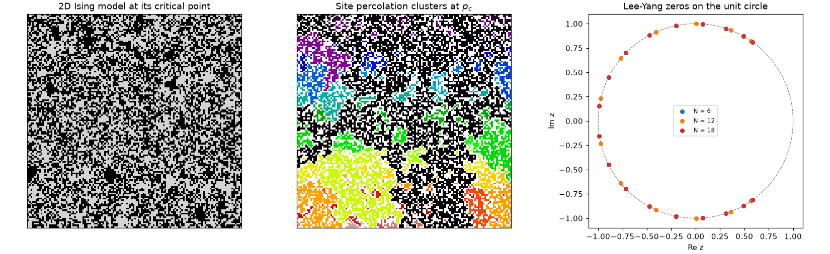

  

Shared infrastructure, used across the subpackages above rather than standalone toolkits:

• physicskit.constants -- SI physical constants shared across subpackages, plus a few well-defined unit conversions (energy/temperature, eV/joules, gravitational G=1 unit systems).
• physicskit.integrators -- shared numerical ODE integrators (RK4, leapfrog, Yoshida4, adaptive Dormand-Prince) and SDE integrators (Euler-Maruyama, Milstein, BAOAB Langevin) used across the other subpackages.
• physicskit.units -- explicit natural-unit systems (G=1, G=c=1, hbar=1, k_B=1, or any combination) with user-chosen scales, SI conversion, and optional pint interop.
• physicskit.results / physicskit.io -- a shared, unit-aware Result container with adapters for existing subpackage outputs, saved to .npz or HDF5.

Design

physicskit calls numpy/scipy directly for anything they already implement (FFTs, dense and sparse eigensolvers, quadrature, special functions, statistical tests), and hand-rolls an algorithm only where the algorithm's own steps are the pedagogical subject (symplectic and Boris integrators, particle-in-cell, FDTD, Metropolis and Wolff updates, geodesic ray tracing) or where no numpy/scipy equivalent exists (e.g. topological invariants, billiard maps). Time-stepped inner loops are numba-compiled, and the ODE integrators are shared across domains. Each subpackage computes in its field's natural units (astro: G = 1; relativity: G = c = 1; quantum: ħ = 1; statphys: k_B = 1), while physicskit.constants holds the SI values.

Test

Tests live alongside each subpackage, at physicskit/<name>/tests/.

pytest                                              # everything
pytest physicskit/rmt/tests                         # a single subpackage

# docstring examples, across every subpackage (pyvista's 3D viewer is
# optional and skipped rather than installed as a hard test dependency):
MPLBACKEND=Agg pytest --doctest-modules physicskit \
    --ignore-glob="*/tests/*" \
    --ignore=physicskit/chaos/visualizers/viewer3d.py

Both commands, plus ruff check/ruff format --check, run in CI on every PR (.github/workflows/ci.yml) across Python 3.10-3.15 on Linux and macOS, as does mypy on the whole package. See CONTRIBUTING.md before opening a PR.

Performance benchmarks for the shared integrators and three representative solvers live in benchmarks/:

pip install -e ".[bench]"
pytest benchmarks

Coverage

MPLBACKEND=Agg pytest -q -n auto --cov=physicskit --cov-report=term

CI measures coverage on every push and PR and uploads it to Codecov, which drives the badge above; the per-file table is also written to each CI run's job summary. Modules outside visualizers/ aim for full line coverage. visualizers/ modules are smoke-tested only (correct return type/shape, or that anim.save() succeeds) rather than covered line-by-line, per the testing convention in CLAUDE.md, so subpackages with large visualizer modules (chaos, quantum, statphys) report lower overall numbers. @njit-compiled lines are excluded from coverage entirely (pyproject.toml, [tool.coverage.report]) since coverage.py cannot trace into numba-compiled native code.

Docs

Built docs are hosted at https://cpoli.github.io/physicskit/, served from the gh-pages branch, which CI redeploys on every push to main and on each release. To build locally:

pip install -e ".[docs]"
cd docs && make html

See docs/source/history/ for a chronology of each field's foundational breakthroughs, linked to the corresponding implementation at each step. The README figures are regenerated with python docs/make_readme_figure.py and python docs/make_readme_subpackage_figures.py.

Long-form tutorials, including a "Units and conventions" guide to each subpackage's natural units, are in docs/source/tutorials/.

Citation

If you use physicskit in your research, please cite it — see CITATION.cff.

Contributing

See CONTRIBUTING.md. Please note that this project follows the Contributor Covenant.

License

MIT -- see LICENSE.